1 Introduction

Production networks are highly transient, variable and unavailable to serve as testbeds for algorithmic development. A wireless link that is lossy today is clean tomorrow, an LTE cell measured at 9 a.m. is congested by noon, and no operator will hold an impairment steady long enough for an algorithm to settle into a stable regime. A run taken on Tuesday cannot be compared against one taken on Wednesday, because the path may have re-routed. The difference the developer cares about, the one the code change produced, is routinely smaller than the difference the network produced on its own. Emulators can recover part of the control by injecting impairments on a physical NIC but failure is still hard to model and harder still to capture. WarpSIM was built to repeatably surface success, failure, and internal algorithm state so that detailed and complex interactions between components could be studied.

Developing a congestion-control algorithm needs three capabilities.

The first is fine grained visibility. A packet capture shows what a sender emitted; it does not show why. The estimator inputs the algorithm used, the thresholds it compared them against, the phase it was in, and the instant each of those changed are what the developer needs. WarpSIM was thus built to capture, events, metrics algorithm values at the times that they change. Furthermore, it was engineered to add new metrics in the future so that algorithmic changes were easy to monitor.

The second is reproducibility. Judging whether a change helped, or noticing that it regressed, requires two runs that differ only in the code under test. The run along with its initial packet injection must be a repeatable function of its configuration and its seed. Any environmental factors and source of randomness not under test need to be eliminated.

The third is portability. A run must reproduce independently of the hardware it runs on, so teams can compare results without accounting for differences between test platforms. WaprSIM is built and engineered to be host platform agnostic and due to its generic Python implementation can run on any host that can run Python 3.12 or better.

WarpSIM is a pure discrete-event simulator designed around these capabilities. It hosts kernel-faithful and specification-faithful CC implementations and router queueing disciplines on a common kernel-style harness; it carries logical time as integer picoseconds, eliminating the drift a floating-point clock would accumulate in billion-event runs; it records all events and their associated actions; and it can be calibrated against live captures (Section 8). The last one is important. Calibration against real environments was instrumental in honing our algorithms prior to moving to live infrastructure deployments. Also, just as important, faithful real-world reproduction of network behavior provides confidence that algorithms under test will perform faithfully in production.

In order to achieve faithful simulated reproduction of real network environments, WarpSIM models the IP layer and above in software, together with the host’s offload

quanta: the paced sender’s TSO chunking, the receiver’s GRO aggregation and SACK compression, and the host-mode queueing discipline that paces every flow on a deployed origin (Section 5). It does not model TLS handshake costs, host OS scheduling, or radio-layer scheduling beneath the loss, jitter, capacity-variation, and ACK-channel abstractions its link and endpoint models provide. Researchers needing radio-layer fidelity should look at ns-3’s LTE module or a hardware testbed.

2 Related Work and Tools

Simulators. ns-3 [1] is the dominant academic simulator, C++ based, with extensive radio-layer models and a deep library of contributed CC implementations. Its practical costs are setup complexity and a conservative pace of upstream CC updates¹. For radio-layer-deep questions ns-3 remains the right tool; for transport-only questions at modern wire speeds across multi-billion-event runs, the configuration effort outweighs the benefit. htsim [2], from the original DCTCP and MPTCP teams, is fast and deterministic but models data-center fabrics rather than last-acre impairments. OMNeT++ [3] with INET offers comparable fidelity at a similar configuration cost.

Emulators. Mininet [4] runs real Linux stacks in namespaces, which makes it right for correctness questions about end-to-end behavior and wrong for quantitative ones at wire speed, since the host’s own scheduling jitter dominates whatever the researcher is trying to isolate. Mahimahi [5] records and replays captured paths rigorously, but it is limited to the conditions in the recording, so it cannot walk an impairment axis end to end, which is the experiment WarpSIM exists for. netem with tc is the default for one-off experiments, and its reproducibility is limited by host scheduling when data rates exceed 1 Gbps.

Hybrid and hardware. Pantheon [6] is closest in intent, running one CC across emulated, simulated, and live paths; its breadth of CCs and paths is the strength and the configurability of its impairments the weakness, since it inherits them from whichever mode the researcher selects. Hardware testbeds are the right tool when the radio must be real, and the wrong one for “what does CC X do under exactly 5% loss for two million packets?”, because real radios do not produce exactly 5% loss on demand.

Methodology and artifacts. Pantheon’s cross-tool comparison reports simulated and live results agreeing to within roughly 20% for most CCs, which is where the calibration target of Section 8.3 starts; the agreement reported there runs tighter because the path selection is narrower and the impairment models are deduced from specific captures rather than from a generic class. The TCP Evaluation Suite [7] standardized a benchmark corpus without prescribing a simulator, and WarpSIM’s sweeps cover most of its scenarios. Our calibration discipline follows the pattern ns-3’s Wi-Fi validation [8] established: configure from a capture, run a reference algorithm, and attribute the residuals. The release targets the artifact criteria of SIGCOMM [9] and NSDI [10].

The implemented calibration paths are anchors rather than a representative sample of the public internet, and folding broader characterizations (CAIDA [11], M-Lab [12]) into the impairment models is future work.

3 Design Goals

Three design goals drove WarpSIM’s architecture, and each ruled out alternative designs.

3.1 Determinism and Replay

Whenever a test is repeated using the same control inputs and algorithm WarpSIM must produce an identical result deterministically. The determinism allows a meaningful comparison of different algorithms. Given the same configuration and random seed WarpSIM will generate an identical packet event sequence thereby enabling algorithm evaluations.

This capability requires three design rules:

1. Simulated time must be exact.
2. Isolate simulated time from real time.
3. Assign per-trial pseudo-random seeds and re-use them for each trial re-run.

The 3 rules force simulated time to be tracked as an integer count of picoseconds and be independent from wall time. By conforming to the rules WarpSIM allows a run to be repeated without saving its entire event history. Large batches of tests thus record only summary results. When a result needs investigation, that test can be repeated with detailed logging enabled. The log can then record each event’s source, destination, type, packet size, queue timings, and internal simulator state. Only the runs worth investigating incur the storage cost of a full trace. Replay is thus effectively free except for the time it takes to redo a trial run.

3.2 Throughput for Parameter Sweeps

A typical evaluation includes six impairment-axis sweeps (jitter, loss, RTT, link speed, convergence time and wireless burst models), each evaluated across multiple CCs at twenty or more impairment levels with five seeds each. That is roughly 2,400 individual runs per sweep set, and multi-flow fairness work generates a comparable volume.

WarpSIM was profiled and tuned to run a 60-second simulated scenario in under a minute of real wall-clock on a single core, so a full sweep set completes in hours rather than days once the runs are distributed. The architecture decisions that make this possible (event queue representation and node dispatch model) are covered in Section 4.

3.3 Visibility

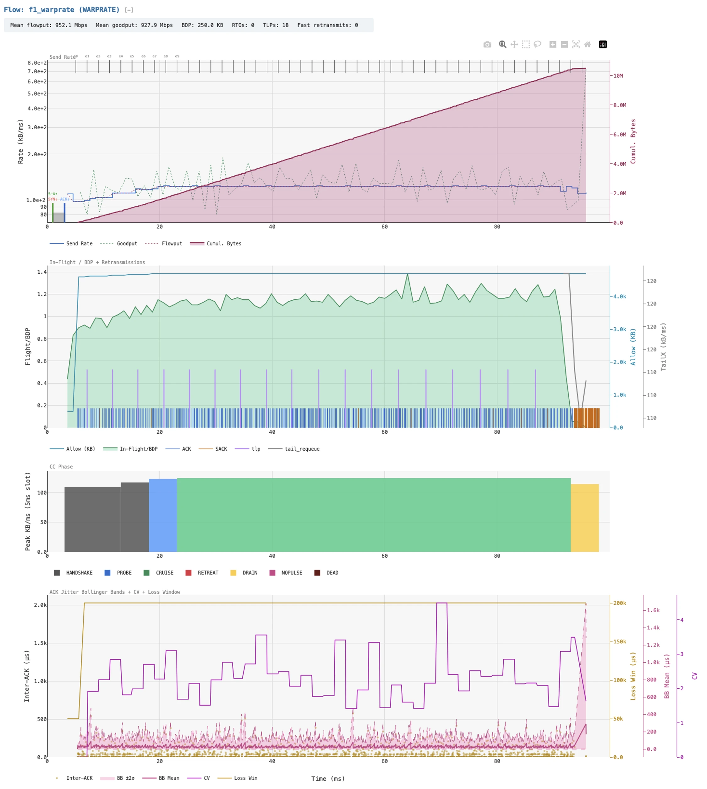
A trial trace is often millions of events, and a CC’s mistakes are rarely visible in a table of them. WarpSIM was designed so that the researcher sees each algorithm’s reasoning plotted against the packets it produced. Every run writes a self-contained HTML report whose per-flow panels share a common time axis. The report plots send rate, goodput, in-flight bytes against BDP and the CC’s ceiling, the CC’s phase timeline, its estimator state, and marks the plot with ACK, SACK, TLP, and retransmit events drawn as individual marks (Figure 1).

The CC interface exposes those internal variables to the harness, so the plots

show the algorithm state when it acted, not a post-facto reconstruction from a logged packet trace. While a packet capture can show that a sender slowed down; the CC’s internal state shows which estimate told it to do so.

Multi trial sweeps are cataloged one level up, with each impairment axis rendered as a line or bar chart of goodput per CC, so the trial where one algorithm diverged can be isolated and then opened in its per-flow view.

4 Architecture

The WarpSIM architecture is organized around three abstractions: time (carried as integer picoseconds on every event), the event queue (a binary heap with monotonic-counter tie-breaking), and the engine loop (pop event, advance simulated time, dispatch to event handler, repeat). The rest of this section covers each and the design choices behind it.

4.1 Time as Integer Picoseconds

Logical time is a Python int and represents picosecond precision, carried as an absolute timestamp on every event; the engine’s clock advances to the next event’s timestamp on each iteration. The unit is chosen for headroom and exact conversion: a 100 Gbps link serializes a 1500-byte segment in 120 nanoseconds while a 1.2 Tbps link serializes that in 10 nanoseconds. Since sub-microsecond Gaussian jitter produces sub-nanosecond quantities, picoseconds let every model remain time-exact up to terabit data rates. Furthermore, integer arithmetic is deterministic across runs, platforms, and Python versions, where a float clock would be order-dependent. Profiling puts the cost of arbitrary precision in the noise, since the relevant magnitudes fit in 64 bits and Python’s int implementation optimizes such transparently.

4.2 The Event Queue

The event queue is a min-heap keyed on (abs_time_ps, monotonic_counter). The monotonic counter is a per-process integer that increments on every schedule(event) call and serves as a FIFO tie-breaker for events that share a timestamp. While rare, without the counter, two events with equal timestamps would make heapq compare the event objects themselves, which are not orderable, and the order of tied events would be undefined.

The interface is intentionally small:

schedule(event): insert into the heap.

pop(): remove and return the earliest-scheduled event.

peek_time(): inspect the next timestamp without dequeue.

is_empty(): termination condition for the engine loop.

The implementation wraps heapq. We profiled calendar-queue alternatives, which trade asymptotic worst-case behavior against the heap’s expected-logarithmic behavior, and found that the heap is best for the workloads WarpSIM is built for. The calendar queue’s structure is preferable for very-large-N steady-state simulations, which is not the operating regime of CC research.

4.3 The Engine Loop

The main loop is the simplest part of the simulator:

while not event_queue.is_empty():
    event = event_queue.pop()
    if event.cancelled:
        continue
    current_time_ps = event.abs_time_ps
    nodes[event.target_node_id].handle(event)

A cancelled timer stays in the heap and is skipped when it is popped. A node’s handle is a typed dispatch: it calls event.event_type.dispatch(node, event), where the event type is a DEnum value from the JEnum library and dispatch is a method on the enum constant that invokes the matching handler on the node.

The engine terminates when the queue empties or when a configured simulation-time horizon is reached. On a typical CC experiment the queue empties naturally as the simulated transfer completes; horizon termination is reserved for steady-state experiments and stability sweeps.

4.4 The Topology Graph

The simulated network is a directed graph whose vertices are nodes and whose edges are links. Nodes carry their own state machine and a typed handle(event) method; links are physical FIFO pipes parameterized by bandwidth (bits per second), one-way propagation delay (picoseconds), and per-direction loss and jitter models. Links preserve packet ordering, so packets exit in the order they entered, and multiple packets may be in flight at once.

The graph is constructed from a JSON topology configuration. The configuration specifies nodes by type (endpoint, router, switch, WarpEngine proxy), links by endpoints and parameters, flows by source/destination/start-time/size, and the simulator’s runtime parameters (RNG seed, horizon, log verbosity). Thus a single configuration file plus the master RNG seed fully specifies a run, which is what the determinism goal of Section 3 requires.

5 Node and Link Models

WarpSIM models a small set of node types and a parameterized link model. Single and multi-node topologies are supported including multiple links in and out of the same node. WarpSIM implements functional kernel parity such that algorithms tested in simulation context mirror their behavior in production deployments with high fidelity.

5.1 Endpoints

An Endpoint is a TCP sender or receiver, with its state machine implemented in Python. Receivers generate cumulative and SACK acknowledgments, maintain a receive

buffer parameterized by RWND, and emit ECN echoes when CE marks arrive; senders maintain a send buffer, manage retransmission state, drive a pluggable CC, and reach the SACK and ECN machinery through the kernel-style interface of Section 6.

The implementation follows the Linux kernel rather than the RFC text, because the live comparisons the simulator is calibrated against run on that kernel. The endpoint carries SACK and ECN, and it takes RTT samples from both timestamps and SACKed segments. Loss detection is RACK-TLP [13] with the kernel’s reorder window and reordering detection, which raises the duplicate threshold toward the reordering distance it observes. Loss-based CCs recover through PRR (RFC 6937), with F-RTO (RFC 5682).

Handshake segments are retransmitted with exponential backoff. The receiver reproduces the kernel’s ACK timing. It runs in quick-ACK mode, ACKing every segment, for the first 16 segments and after out-of-order data, and otherwise delays ACKs with the 40 ms TCP_DELACK_MIN floor. The send buffer bounds the data in flight as sk_sndbuf does in the kernel. Stock CCs keep the kernel’s default 4 MB ceiling, and WarpRATE runs without one, because its deployment sizes the buffer per socket [14].

5.2 Routers and Queueing Disciplines

A Router has one or more input and output ports, each carrying a queueing discipline selected at configuration time. Five queueing disciplines are implemented: FIFO with tail-drop, CoDel [15] at its 5 ms default target, FQ-CoDel [16] adding per-flow scheduling on stochastic hashing, DualPI2 [17] for L4S coupled marking across a classic and a scalable queue, and PFQD [18], ported from the sch_pfqd kernel module.

CoDel and FQ-CoDel implement typical defaults and state variables, and every discipline enforces a port’s buffer limit as its kernel counterpart does. Where a router has several ports toward one destination, it forwards on the first by default, by a hash of the flow (ECMP), or by packet, each packet taking a seeded random port, which models the packet spraying of multipath datacenter fabrics.

A Switch is a Layer-2 forwarding element with MAC learning and per-port buffering, present so that data-center and home-network topologies can carry realistic Layer-2 segments instead of collapsing into router hops.

A WarpEngine node is a TCP-terminating proxy that splits a flow into two legs, each running its own CC instance and seeing only its own RTT and impairment profile.

5.3 Links

Beyond the bandwidth, propagation delay, and FIFO ordering of Section 4.4, each Link applies loss, jitter, and capacity variation independently per direction. Loss is Bernoulli with a configurable per-packet probability, Gilbert-Elliott, periodic, or bernoulli_train, a two-state model with a mean train length and an inter-train probability that captures the burst patterns cellular paths produce.

Four of the jitter models are generic: Gaussian with a configurable σ truncated at zero, uniform, Pareto, and periodic burst. Three model specific radio links. The wifi_txop model captures 802.11 CSMA/CA contention as a burst-and-gap pattern, parameterized by burst interval, within-burst σ, and burst size. The lte_subframe and 5g_nr models quantize arrivals to a configurable subframe or slot boundary. Two models reproduce reordering. The netem model is symmetric about a mean and reorders packets as Linux netem does, and reorder holds back a fraction of packets so later ones overtake them.

Capacity variation is a dwell process on the service rate. It can optionally add heavy-tailed dips fitted from live ACK streams, a demand-responsive grant ramp for radio schedulers, and scheduled outages. Every model draws from a per-direction seed derived from the master seed, so direction-specific behavior reproduces independently of the rest of the run.

5.4 Host and Receiver Offload

A real-world sender does not put packets on the wire one at a time, and thus the simulator does not either. A paced sender emits TSO chunks of pacing_rate / 1024 / MSS segments per pace tick, floored at two segments and capped at the 64 KB GSO limit, following the kernel’s autosizing rule. A pfqd node marked host_mode runs as the origin’s egress qdisc and paces each flow at its CC’s rate. A CUBIC sender model is thus host-paced as it is on a deployed server.

On the receive side, the simulator reproduces the ways a real path bulks ACKs. A receiver with GRO configured aggregates back-to-back in-order arrivals of a flow into one receive event and makes one ACK decision per aggregate, with the coalescing interval and aggregate cap set per flow: a NIC interrupt window on a wired host, an A-MPDU on WiFi, a scheduling interval on LTE or 5G.

The receiver also compresses SACKs after the third duplicate as the kernel does, and it can advertise its receive window as the kernel’s autotuning grows it, doubling per RTT from an initial value. Three additional models are fitted from live ACK streams. A receive hold delays every data segment’s arrival at the stack by a fixed interval, reproducing the interrupt-coalescing latency seen on wired clients. An ACK-path hold, fitted on the wired trial, holds each pure ACK for a delay drawn from measured quantiles once the flow’s arrival rate saturates the path and releases held ACKs in order, so long holds arrive as clumps of back-to-back ACKs. A handset or a satellite terminal sends ACKs only when the uplink scheduler grants it a transmit opportunity, so its ACK channel is modeled as a grant process. Each medium has its own profile, which sets the quantiles of the gap between grants, how many ACKs each grant releases, how often ACKs are lost, whether the CPE filters ACKs, and how uplink slots quantize them. The profile also carries the receiver’s window schedule for that medium. The grant process draws from a seed derived from the run’s, so a

multi-seed sweep varies it along with everything else. These models exist because, as [19] argues, the offload quanta rather than per-packet timing are what a CC experiences on a modern host.

5.5 Composability

A “p-rtr-p” topology is two endpoints with a router between them; “p-we-p” adds a proxy between the router and one endpoint; “p-rtr-rtr-p” adds a second router for an enterprise WAN. Each is an individual JSON file, so moving between them is a configuration change rather than a code change, and a study walking twenty distinct topologies is twenty configuration files.

6 The Congestion Control Interface

WarpSIM’s CC harness mirrors the Linux kernel’s tcp_congestion_ops interface. Each CC implementation is a Python class that overrides a fixed set of hooks invoked by the TCP state machine at well-defined events. The discipline of the interface is what makes cross-CC comparison trace-equivalent at the dispatch boundary: when CUBIC and WarpRATE run on the same scenario, the only behavior that differs is the behavior inside their CC hooks, because every other piece of TCP machinery is shared code.

Mirroring the kernel interface keeps a new CC small: about 200 lines of Python suffice for a loss-based or delivery-rate-based CC, and the hooks map one to one onto a kernel module’s. CC selection is a per-flow parameter in the JSON topology, so a simulation can run flows with different CCs over the same path, and the harness ensures each flow’s CC sees only its own state, which is what mixed-CC fairness experiments on a shared bottleneck require.

6.1 Instrumentation Hooks

Every hook the CC overrides is also a logging point. The simulator’s trace output includes the CC’s name, the hook fired, the inputs to the hook, and the resulting state change. For CCs that expose additional internal signals (e.g. WarpRATE’s per-epoch delivered volume, BBR’s BtlBw filter window, DCTCP’s α), the CC implementation registers those signals at init time and the simulator’s trace emitter logs them on each update. The result is a per-flow time series of every signal the CC consumed and every decision it made.

7 Reference CC Implementations

WarpSIM ships five congestion-control implementations using the harness outlined in Section 6. This section documents the important details of each.

7.1 CUBIC

CUBIC is a port of the kernel’s tcp_cubic.c, which implements RFC 9438 [20]: the Ha-Rhee cubic growth function [21] $\text{CWND}={𝐶\left(𝑡-𝐾\right)}^3+{𝑊}_{\{max\}}$ at the core, the fast-convergence refinement [[20], §4.6] that biases recovery toward a smaller ${𝑊}_{\{max\}}$ when consecutive losses are detected, and the TCP-friendly region [[20], §4.2] that preserves Reno-compatible behavior on short-RTT links. Slow start exits on the kernel’s HyStart, with both its ACK-train and delay heuristics enabled as in the kernel default. Loss detection and recovery are the endpoint’s kernel machinery of Section 5.

7.2 BBR

The implemented BBR is a port of the v3 kernel module (google/bbr branch v3), with the windowed-max BtlBw filter, the four-phase machine of STARTUP, DRAIN, PROBE_BW, and PROBE_RTT of the original publication [22], and v3’s explicit inflight caps, the inflight_hi loss bound, and the ECN and loss lower bounds. Each kernel function has a named counterpart, and the port was audited function by function against the module source.

7.3 DCTCP

DCTCP [23] implements the proportional CE-mark response indexed by the EWMA marking fraction $𝛼$, with the $\frac{𝛼}{2}$ multiplicative window reduction on each round. The implementation assumes the bottleneck qdisc supports ECN with a configurable RED-style marking threshold; on a non-marking qdisc it starves, which is the specified behavior rather than an implementation artifact.

7.4 Prague (L4S)

Prague [24] tracks the IETF draft, including the RTT-independence response and the scalable marking behavior that distinguishes it from DCTCP off data-center paths. It is normally paired with DualPI2 [17] under the L4S architecture [25].

7.5 WarpRATE

WarpRATE [26] is a port of the tcp_warprate kernel module, about 2,200 lines of Python that use the kernel’s constants and write per-epoch records under the kernel’s field names, so a simulated trace and a live one read the same way. The simulator is kept at parity with the module through a tracked backlog of sim-to-kernel differences, and a mechanism the kernel retires is deleted from the simulator rather than kept behind a switch, so a trial cannot be measured under a law the kernel no longer runs. A warprate_rttvar variant ships for RTT-variance studies. WarpRATE’s instrumentation requirements drove the trace schema described in Section 9.

7.6 Variants

Three further CCs ship for specific studies: WarpTCP, the CUBIC-based predecessor of WarpRATE deployed in split-connection proxies; BBRB, BBRv3 with the smoothed-RTprop correction Kumar et al. propose [27]; and a constant-rate pump for link tests. Each is selected by name in the JSON configuration.

7.7 Adding a New CC

To add a new CC implementation: subclass the CongestionControl base class, override the hooks that diverge from the default Reno behavior,

register any CC-specific signals for trace emission, and add a JSON config entry mapping the CC’s name to its module path.

8 Calibration Methodology

A simulated path is only as useful as its correspondence to a real one, and that correspondence has to be established against CCs whose real behavior is already known. If sim BBR does not match real BBR on a real path, no simulated result for a new algorithm on that path is informative. Calibration is the procedure that establishes the correspondence. Section 8.1 outlines the method and Section 8.2 discusses its use.

8.1 Method

Capture. Record live transfers on a representative path with each CC the simulator implements and that is of experimental interest. Ideally, the captures should be interleaved so that all of them experience similar network conditions over several runs each. The goal is to record the sender’s internal state sampled per millisecond (RTT, RTT variance, delivery rate, pacing rate, congestion window, retransmits). Where the CC exports per-ACK or per-epoch telemetry, record that also. A client-side packet capture serves as an independent check on what the receiver processed. Along with the traffic, note both endpoint configurations: namely, the server’s qdisc and send buffer settings, the initial window, and the application’s write pattern.

Deduce. The next step is to reduce the capture and infer the parameters of the path and the receiver. We will need bandwidth, RTT both min and average, buffer depths, jitter in both directions, loss patterns, and rates of transmission. Use the average and epoch measured delivery volume to compute maximum and peak bandwidth, min and average RTT. Use the variance of ACK’s to estimate jitter, use the prevalence of SACK’s to estimate re-ordering and loss. These are then mapped to appropriate WarpSIM parameters so that a comparable simulated path behavior can be configured.

Configure and replay. Enter the deduced parameters along with a network topology specification into a JSON config file and simulate the captured transfer size with corresponding CC algorithms across several fixed seeds. A simulation is reproducible from its seed, so any run can be re-examined later with full logging.

Compare. Align clocks at the first data byte, then compare the time taken to deliver fixed milestones (10 MB, 100 MB) as well as overall goodput. Ideally, the simulated transfer should match within 10-20% of the captured transfer. Compare the internal state the same way: retransmits, the distribution of RTT over its floor, and any CC telemetry that both sides record. Try not to overmatch, sometimes network conditions are transient and difficult to infer actual causes from.

Admit and extend. A trial is ready for a CC under development once the stock CCs match to live within a desired factor. Matching stock CCs does not constrain every mechanism of a path, though, and a new algorithm that uses a signal its predecessors ignore can diverge on a trial where CUBIC and BBR agree. The new CC’s telemetry must then becomes part of the capture. The discrepancy shows which mechanism the trial is missing, and the fix follows the Compare step: add the mechanism as a path or receiver model, fit it from the capture, and confirm that the stock CCs still match.

8.2 Example: A Wired ISP Path

The trial in this example models a browser on a fixed ISP line, downloading over HTTP/1.1 from one of our origins running Linux 6.14. It was fitted from 57 traces providing server-side TCP_INFO records of CUBIC and BBR capturing behavior on the path and using it to create a simulated network with similar properties. The network was then used, first for simulation, and later for live results back confirmation.

Capture. The reference set was ten further live sweeps on the same line, each running CUBIC, BBR, and WarpRATE back to back. Neither set included a client-side packet capture.

Table 1: Wired ISP trial, sim against live

	t10 ms	t100 ms	Goodput Mbps
CUBIC sim	518	1,601	589
CUBIC live	525	1,700	540
BBR sim	556	1,677	569
BBR live	525	1,650	595
WarpRATE 3.9.7 sim	758	2,554	500
WarpRATE 3.9.7 live	750	2,600	515
WarpRATE 3.9.8 sim	374	1,554	595
WarpRATE 3.9.8 live	426	1,576	587

Configure. Analysis showed a 690 Mbps bottleneck (peaks of 740–800) from BBR’s delivery rate, a 34.6 ms propagation floor, and a 12 MB buffer from CUBIC’s largest smoothed RTT. TCP_INFO showed an initial window of 10 segments, and the origin’s send buffer was 16 MB. The receiver’s window started at 128 KiB and doubled each round trip to 16 MB. The client acknowledged in 6.5 ms batches. Above about 550 Mbps the client also held some ACKs back, by up to 110 ms, and released them in order as a clump; the simulated trial reproduces this with a per-ACK hold whose delays follow a distribution whose parameters were measured from WarpRATE’s per-ACK records on the live runs.

Verify. The top four rows of Table 1 compare the stock CCs in the simulator with the live median of the ten sweeps, on the TCP_INFO clock. Both reach 10 MB and 100 MB within 6% of live, and their goodput lands within 10%, so the trial was admitted.

Test the new CC. The same live sweeps showed WarpRATE release 3.9.7 at 515 Mbps against BBR’s 595. Replayed on the trial, sim WarpRATE reproduced the shortfall, reaching 10 MB at

758 ms against 750 live. The per-flow visual view located the cause in WarpRATE’s startup [26]: the origin paused about 100 ms between its connect frames and the response body, and the startup rule read that application silence as evidence of a batching path and settled on a low initial pacing rate. A candidate fix, counting a silence only while data is in flight, raised sim WarpRATE to 595 Mbps and brought its 10 MB time to 374 ms.

Confirm live. The fix shipped as release 3.9.8, and ten live sweeps on the same line that evening measured WarpRATE at 587 Mbps and 1,576 ms to 100 MB, against the simulator’s 595 Mbps and 1,554 ms, both within 2%. The 10 MB time came in at 426 ms against the predicted 374, so the simulator was 12% optimistic. In that particular session WarpRATE moved from 0.87 of BBR’s live goodput to 0.99.

8.3 Coverage

The method of Section 8.1 has been applied to 18 live trials. Their paths were chosen to span the impairment dimensions catalogued in [19]: clean long- and medium-haul wired paths, a very-long-RTT path with bursty loss, a cellular path, an 802.11 path, and a LEO satellite path, each captured under fq, fq_codel, and pfifo_fast at the server egress in separate runs. Implementations with no live reference are anchored to published data, DCTCP to the data-center testbed of [23] and Prague to the L4S evaluation of [28].

The initial acceptance band was agreement within 20% of captured goodput, on the reasoning that a simulator inside that band supports qualitative and comparative claims about CC behavior. Sim BBR reproduces the production kernel within 16% of reference goodput in 13 of the 18 region-by-qdisc trials, and the remaining implementations reproduce their anchors, most within 10%.

9 Fidelity and Flow-Level Visibility

Goodput agreement admits a trial (Section 8), but it is not the fidelity that developing a congestion controller needs. An algorithm fails through its internal state: an estimate taken from a distorted sample, a phase entered at the wrong moment, a signal the path does not produce the way the design assumed. Developing, modifying, and validating a CC therefore requires seeing that state at the resolution the algorithm acts on, every ACK and every epoch, and seeing it the same way in the simulator and in production. WarpSIM records each variable a CC reads at the instant it reads it, and WarpRATE’s kernel module exports its per-epoch records under the field names the simulator writes (Section 7), so a simulated trace and a live one can be compared side by side.

Figure 1 is the standard per-flow view the harness emits for every run. Its four panels share one time axis. The first carries send rate, goodput, and cumulative bytes, with epoch boundaries ticked along the top. The second plots in-flight bytes against BDP and the CC’s own in-flight ceiling, with ACK, SACK, TLP, and tail-requeue events drawn underneath as individual marks. The third is the CC’s phase timeline, colored by state. The fourth shows the sender’s jitter estimator when the CC has one: the inter-ACK samples, the band around them, and the interval they drive. Every quantity in the view is recorded rather than reconstructed from a packet capture.

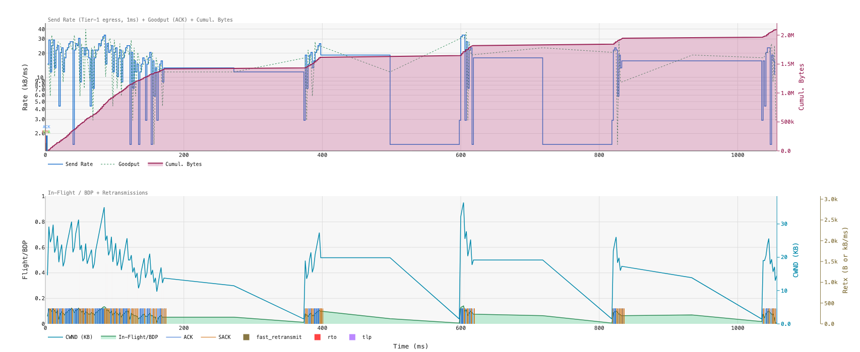
That depth is what makes triage quick. Figure 2 shows the first two panels for CUBIC on a lossy path, where the window sawtooth, the retransmit raster thickening under scatter loss, and the recovery periods that leave the path mostly empty sit in one frame, so the shortfall reads as loss recovery before anything else is considered. A similar analysis located WarpRATE’s startup shortfall in Section 8.2: the phase timeline showed the startup settling at a low rate immediately after the origin’s pause, the candidate fix was explored in the simulator, and the release that carried it matched the simulator’s prediction when live.

Fidelity at that depth also exposes the path. On the same trial sim CUBIC matched live while sim WarpRATE did not, and the server’s TCP_INFO could not say why, because a per-millisecond sample averages over the ACK stream. WarpRATE’s per-ACK records showed the client acknowledging on its receive-offload clock, coalescing arrivals through GRO and releasing ACKs in grants, and those records became the models of Section 5.4. A CC that reads finer signals than its predecessors needs a trace at least as fine as those signals: triage happens on the view, options are explored in the simulator, and the chosen fix moves to production with the same records there to confirm it.

10 Use Cases

WarpSIM has been used for three classes of experiment that live networks cannot easily support.

Multi-flow scheduling studies. Queueing-discipline work needs a workload that live hardware cannot hold stable: 3, 8, 16, and 32 simultaneous flows on a shared bottleneck, each flow’s CC drawn from a configured mix, under each of the five queueing disciplines. A sweep of that shape runs to roughly 1,500 individual runs, completes in about four hours on a single workstation, and preserves every per-flow trace for follow-up analysis.

Re-evaluating published results. Kumar et al. [27], motivated by mmWave links, show BBR’s

throughput collapsing on an emulated 1 Gbps path when netem adds normally distributed delay with a 5 ms mean and σ of 0.5 to 1.25 ms: early packets pull the windowed minimum RTT below half the mean, CWND falls below the BDP, and the bandwidth estimate follows it down. Their testbed ran BBR v1. Re-running their layout on the BBRv3 port, with a jitter model that reproduces netem’s symmetric delay and reordering, shows the same mechanism at larger σ and with less damage.

Across their range BBRv3 holds 938 to 962 Mbps, its minimum RTT still just above half the mean. At σ = 2 ms the estimate falls to a third of the mean and CWND to the BDP, at 862 Mbps; at 3 ms it falls to a fifth, CWND drops below the BDP and throughput settles at 595 Mbps, a 38% loss where Kumar measured 95% for v1. Their smoothed-RTprop correction, run as BBRB, holds 961 Mbps at every σ but keeps the 1000-packet buffer full, with 3,700 to 14,500 retransmissions per 10s run where BBRv3 has none.

Impairment-axis sweeps. Holding every variable fixed but one, walking that one end to end, and recording each CC’s response is the experiment live infrastructure cannot supply, because it cannot hold the impairment constant for the duration of every run in the sweep. Jitter magnitude, loss rate, RTT, link speed, time-to-convergence, and wireless burst pattern are each such an axis. Production network operators also will not run the high-jitter and high-loss conditions these sweeps include.

Without WarpSIM, or something close to it, these types of experiments are impossible to perform and reason about. To do so, you must be able to hold the experimental conditions constant over many trial runs and you must have control to vary certain parameters while holding others fixed.

11 Performance

WarpSIM is pure Python and single-threaded, trading raw speed for implementation clarity and for the determinism that any parallel discrete-event core would compromise. On one core of an Apple M2 Max it processes about a million events per second on a typical CC comparison, from 1.6 million on a single 1 Gbps flow down to 410 thousand with 32 flows through a router, so a 60-second scenario at 1 Gbps and 30 ms RTT finishes in about 40 seconds of wall-clock. Sweeps parallelize across runs instead: the sweep mode distributes independent runs over a process pool, and a thousand-point impairment axis completes in about 30 minutes on twelve cores. Memory peaks near 250 MB for a 10 MB single-flow transfer and near 2 GB for 32 flows, most of it the per-packet event log.

Calibration matches the captured paths at the level of goodput and the sender’s internal state, not packet for packet, so event timing inside a flow need not line up with the kernel’s. The calibration anchors span 50 Mbps to 10 Gbps and 2 ms to 230 ms of RTT; outside that envelope the relationships are plausible but unvalidated.

12 Conclusion

Developing a new congestion controller needs a path that holds still and an algorithm whose reasoning can be surfaced and visualized. The usual tools give one or the other. Emulators such as netem, Mininet, and Mahimahi run a real stack over a bulk transfer, which suits confirming that a finished CC behaves, but above 1 Gbps the host’s scheduling perturbs the timing under study, no run repeats exactly, and the CC’s estimator inputs stay hidden behind ad-hoc tracing. Neither predicts whether a change helped. WarpSIM combines integer-time determinism with kernel-faithful stock CCs, calibration against live captures, and a view of the CC’s internal state against its packets on one time axis, and we are not aware of another environment that offers that combination. The tool has thus far been a success and we expect to use it further in network related algorithm work.

References

• [1] G. F. Riley and T. R. Henderson, “The ns-3 Network Simulator,” in Modeling and Tools for Network Simulation, Springer, 2010, pp. 15–34.
• [2] M. Handley, C. Raiciu, and others, “htsim Network Simulator.” 2017.
• [3] A. Varga and R. Hornig, “An Overview of the OMNeT++ Simulation Environment,” in 1st International Conference on Simulation Tools and Techniques (SIMUTools '08), 2008.
• [4] B. Lantz, B. Heller, and N. McKeown, “A Network in a Laptop: Rapid Prototyping for Software-Defined Networks,” in 9th ACM SIGCOMM Workshop on Hot Topics in Networks (HotNets-IX), 2010.
• [5] R. Netravali et al., “Mahimahi: Accurate Record-and-Replay for HTTP,” in 2015 USENIX Annual Technical Conference (USENIX ATC '15), 2015, pp. 417–429.
• [6] F. Y. Yan et al., “Pantheon: The Training Ground for Internet Congestion-Control Research,” in 2018 USENIX Annual Technical Conference (USENIX ATC '18), 2018, pp. 731–743.
• [7] D. Hayes, D. Ros, L. L. H. Andrew, and S. Floyd, “A Common TCP Evaluation Suite,” Internet-Draft draft-irtf-iccrg-tcpeval-01, 2014.
• [8] G. Pei and T. R. Henderson, “Validation of OFDM Error Rate Model in ns-3,” technical report, 2010.
• [9] ACM SIGCOMM, “ACM SIGCOMM Artifact Evaluation.”
• [10] USENIX NSDI, “USENIX NSDI Artifact Evaluation.”
• [11] CAIDA, “The CAIDA Anonymized Internet Traces Dataset.”
• [12] Measurement Lab, “M-Lab: The Measurement Lab Open Internet Measurement Platform.”
• [13] Y. Cheng, N. Cardwell, N. Dukkipati, and P. Jha, “The RACK-TLP Loss Detection Algorithm for TCP.” RFC Editor, Feb. 2021. doi: 10.17487/RFC8985.
• [14] D. Vadura, “WarpRATE: Implementation, Deployment, and Validation on Live Networks,” technical report, 2026.

• [15] K. Nichols, V. Jacobson, A. McGregor, and J. Iyengar, “Controlled Delay Active Queue Management,” RFC 8289, 2018.
• [16] T. Hoeiland-Joergensen, P. McKenney, D. Taht, J. Gettys, and E. Dumazet, “The Flow Queue CoDel Packet Scheduler and Active Queue Management Algorithm,” RFC 8290, 2018.
• [17] K. De Schepper, B. Briscoe, and G. White, “Dual-Queue Coupled Active Queue Management (AQM) for Low Latency, Low Loss, and Scalable Throughput (L4S),” RFC 9332, 2023.
• [18] D. Vadura, “Practically Fair Queueing: A Per-Flow Scheduling Discipline for Shared Internet Links,” technical report, 2026.
• [19] D. Vadura, “The ACK Stream No Longer Keeps Time: Jitter and the Erosion of TCP's Congestion Signal,” technical report, Mar. 2026.
• [20] L. Xu, S. Ha, I. Rhee, V. Goel, and L. Eggert, “CUBIC for Fast and Long-Distance Networks.” RFC Editor, Aug. 2024. doi: 10.17487/RFC9438.
• [21] S. Ha, I. Rhee, and L. Xu, “CUBIC: A New TCP-Friendly High-Speed TCP Variant,” ACM SIGOPS Operating Systems Review, vol. 42, no. 5, pp. 64–74, 2008.
• [22] N. Cardwell, Y. Cheng, C. S. Gunn, S. H. Yeganeh, and V. Jacobson, “BBR: Congestion-Based Congestion Control,” Communications of the ACM, vol. 60, no. 2, pp. 58–66, Feb. 2017, doi: 10.1145/3009824.
• [23] M. Alizadeh et al., “Data Center TCP (DCTCP),” in Proceedings of the ACM SIGCOMM 2010 Conference (SIGCOMM '10), ACM, Aug. 2010, pp. 63–74. doi: 10.1145/1851182.1851192.
• [24] K. De Schepper, O. Tilmans, and B. Briscoe, “Prague Congestion Control,” Internet-Draft, 2023.
• [25] B. Briscoe, K. De Schepper, M. Bagnulo, and G. White, “Low Latency, Low Loss, and Scalable Throughput (L4S) Internet Service: Architecture,” RFC 9330, 2023.
• [26] D. Vadura, “WarpRATE: A Rate-Paced CC Solution,” technical report, Mar. 2026.
• [27] R. Kumar et al., “TCP BBR for Ultra-Low Latency Networking: Challenges, Analysis, and Solutions,” in 2019 IFIP Networking Conference (IFIP Networking), IEEE, 2019, pp. 1–9. doi: 10.23919/IFIPNetworking.2019.8816856.
• [28] D. B. Oljira, K.-J. Grinnemo, A. Brunstrom, and J. Taheri, “Validating the Sharing Behavior and Latency Characteristics of the L4S Architecture,” ACM SIGCOMM Computer Communication Review, vol. 50, no. 2, pp. 37–44, 2020.